43 chart data labels excel

Data Labels on Chart Series - Excelguru Applying data labels when the legend is selected will apply data labels to all the series in the chart. Your screen shot of data labels would suggest that the information is in fact the values of the first series rather than multiple #N/As. Select the actual series before applying data labels. Add data labels and callouts to charts in Excel 365 | EasyTweaks.com The steps that I will share in this guide apply to Excel 2021 / 2019 / 2016. Step #1: After generating the chart in Excel, right-click anywhere within the chart and select Add labels . Note that you can also select the very handy option of Adding data Callouts.

Create Dynamic Chart Data Labels with Slicers - Excel Campus Typically a chart will display data labels based on the underlying source data for the chart. In Excel 2013 a new feature called "Value from Cells" was introduced. This feature allows us to specify the a range that we want to use for the labels. Since our data labels will change between a currency ($) and percentage (%) formats, we need a ...

Chart data labels excel

Excel.ChartDataLabels class - Office Add-ins | Microsoft Docs The request context associated with the object. This connects the add-in's process to the Office host application's process. Specifies the format of chart data labels, which includes fill and font formatting. Specifies the horizontal alignment for chart data label. See Excel.ChartTextHorizontalAlignment for details. Excel Charts - Aesthetic Data Labels - tutorialspoint.com To place the data labels in the chart, follow the steps given below. Step 1 − Click the chart and then click chart elements. Step 2 − Select Data Labels. Click to see the options available for placing the data labels. Step 3 − Click Center to place the data labels at the center of the bubbles. Format a Single Data Label Excel Chart Data Labels-Modifying Orientation - Microsoft Community In reply to PaulaAB's post on September 13, 2016. Hi Paula, You can right click on the data label part then select Format Axis. Click on the Size & Properties tab then adjust the Text Direction or Custom Angle. Thanks,

Chart data labels excel. Add a DATA LABEL to ONE POINT on a chart in Excel All the data points will be highlighted. Click again on the single point that you want to add a data label to. Right-click and select ' Add data label '. This is the key step! Right-click again on the data point itself (not the label) and select ' Format data label '. You can now configure the label as required — select the content of ... How to create Custom Data Labels in Excel Charts Create the chart as usual. Add default data labels. Click on each unwanted label (using slow double click) and delete it. Select each item where you want the custom label one at a time. Press F2 to move focus to the Formula editing box. Type the equal to sign. Now click on the cell which contains the appropriate label. Change the format of data labels in a chart To get there, after adding your data labels, select the data label to format, and then click Chart Elements > Data Labels > More Options. To go to the appropriate area, click one of the four icons ( Fill & Line, Effects, Size & Properties ( Layout & Properties in Outlook or Word), or Label Options) shown here. How to Use Cell Values for Excel Chart Labels Select the chart, choose the "Chart Elements" option, click the "Data Labels" arrow, and then "More Options." Uncheck the "Value" box and check the "Value From Cells" box. Select cells C2:C6 to use for the data label range and then click the "OK" button. The values from these cells are now used for the chart data labels.

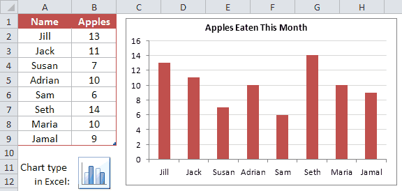
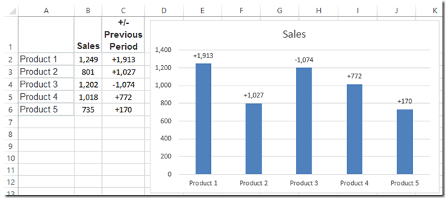
How to Add Data Labels in Excel - Excelchat | Excelchat After inserting a chart in Excel 2010 and earlier versions we need to do the followings to add data labels to the chart; Click inside the chart area to display the Chart Tools. Figure 2. Chart Tools. Click on Layout tab of the Chart Tools. In Labels group, click on Data Labels and select the position to add labels to the chart. Custom Chart Data Labels In Excel With Formulas Follow the steps below to create the custom data labels. Select the chart label you want to change. In the formula-bar hit = (equals), select the cell reference containing your chart label's data. In this case, the first label is in cell E2. Finally, repeat for all your chart laebls. How to Create a Bar Chart With Labels Inside Bars in Excel In the chart, right-click the Series "# Footballers" Data Labels and then, on the short-cut menu, click Format Data Labels. 8. In the Format Data Labels pane, under Label Options selected, set the Label Position to Inside End. 9. Next, in the chart, select the Series 2 Data Labels and then set the Label Position to Inside Base. 10. How To Use Dynamic Data Labels To Create Interactive Excel Charts To create a column chart with dynamic data labels, you need to follow these given steps. Select the data & Create a Combo Chart. Now select the column chart for revenue data and a line chart with marker for data labels Add Data Labels to the Line Chart With Marker. After then remove the Line Color and Marker Color.

What is label in a chart? - Blackestfest.com To format data labels, select your chart, and then in the Chart Design tab, click Add Chart Element > Data Labels > More Data Label Options. Click Label Options and under Label Contains, pick the options you want. To make data labels easier to read, you can move them inside the data points or even outside of the chart. Edit titles or data labels in a chart - support.microsoft.com On a chart, click one time or two times on the data label that you want to link to a corresponding worksheet cell. The first click selects the data labels for the whole data series, and the second click selects the individual data label. Right-click the data label, and then click Format Data Label or Format Data Labels. Move data labels - support.microsoft.com Right-click the selection > Chart Elements > Data Labels arrow, and select the placement option you want. Different options are available for different chart types. For example, you can place data labels outside of the data points in a pie chart but not in a column chart. How to create a chart with both percentage and value in Excel? After installing Kutools for Excel, please do as this:. 1.Click Kutools > Charts > Category Comparison > Stacked Chart with Percentage, see screenshot:. 2.In the Stacked column chart with percentage dialog box, specify the data range, axis labels and legend series from the original data range separately, see screenshot:. 3.Then click OK button, and a prompt message is popped out to remind you ...

E-xcel Tuts: Add Data Labels to Excel Charts

Chart.ApplyDataLabels method (Excel) | Microsoft Docs ApplyDataLabels ( Type, LegendKey, AutoText, HasLeaderLines, ShowSeriesName, ShowCategoryName, ShowValue, ShowPercentage, ShowBubbleSize, Separator) expression A variable that represents a Chart object. Parameters Example This example applies category labels to series one on Chart1. VB Copy Charts ("Chart1").SeriesCollection (1).

How to Add Data Labels in an Excel Chart in Excel 2010 - YouTube

Excel: How to Create a Bubble Chart with Labels - Statology Step 3: Add Labels. To add labels to the bubble chart, click anywhere on the chart and then click the green plus "+" sign in the top right corner. Then click the arrow next to Data Labels and then click More Options in the dropdown menu: In the panel that appears on the right side of the screen, check the box next to Value From Cells within ...

30 How To Label A Chart In Excel - Labels Niche Ideas

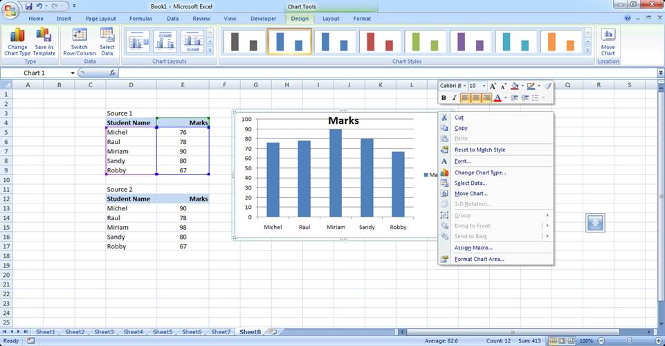
How to Change Excel Chart Data Labels to Custom Values? First add data labels to the chart (Layout Ribbon > Data Labels) Define the new data label values in a bunch of cells, like this: Now, click on any data label. This will select "all" data labels. Now click once again. At this point excel will select only one data label.

Charts and Graphs in Excel

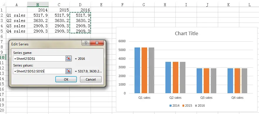
How to add data labels from different column in an Excel chart? Right click the data series in the chart, and select Add Data Labels > Add Data Labels from the context menu to add data labels. 2. Click any data label to select all data labels, and then click the specified data label to select it only in the chart. 3.

Enable or Disable Excel Data Labels at the click of a button - How To - PakAccountants.com

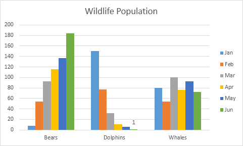
Add or remove data labels in a chart - support.microsoft.com Click the data series or chart. To label one data point, after clicking the series, click that data point. In the upper right corner, next to the chart, click Add Chart Element > Data Labels. To change the location, click the arrow, and choose an option. If you want to show your data label inside a text bubble shape, click Data Callout.

How to Change Excel Chart Data Labels to Custom Values?

Format Data Labels in Excel- Instructions - TeachUcomp, Inc. To do this, click the "Format" tab within the "Chart Tools" contextual tab in the Ribbon. Then select the data labels to format from the "Chart Elements" drop-down in the "Current Selection" button group. Then click the "Format Selection" button that appears below the drop-down menu in the same area.

Excel Gantt Chart - Free Excel Templates

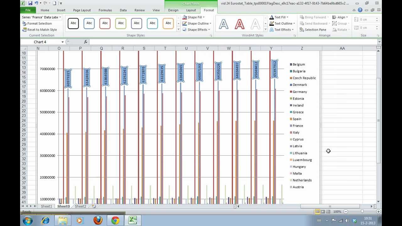
Adding rich data labels to charts in Excel 2013 | Microsoft 365 Blog Data label callouts The data labels up to this point have used numbers and text for emphasis. Putting a data label into a shape can add another type of visual emphasis. To add a data label in a shape, select the data point of interest, then right-click it to pull up the context menu. Click Add Data Label, then click Add Data Callout .

Bar charts with long category labels; Issue #428 November 27 2018 | Think Outside The Slide

Add / Move Data Labels in Charts - Excel & Google Sheets We'll start with the same dataset that we went over in Excel to review how to add and move data labels to charts. Add and Move Data Labels in Google Sheets Double Click Chart Select Customize under Chart Editor Select Series 4. Check Data Labels 5. Select which Position to move the data labels in comparison to the bars.

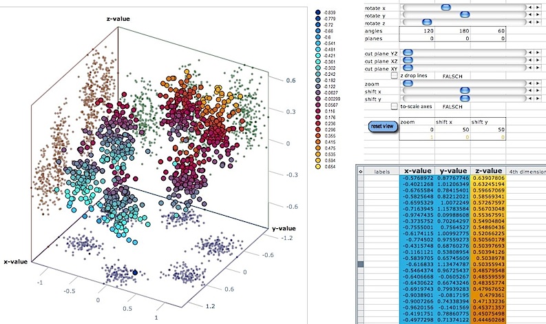
3d scatter plot for MS Excel

How to add or move data labels in Excel chart? - ExtendOffice In Excel 2013 or 2016. 1. Click the chart to show the Chart Elements button . 2. Then click the Chart Elements, and check Data Labels, then you can click the arrow to choose an option about the data labels in the sub menu. See screenshot: In Excel 2010 or 2007. 1. click on the chart to show the Layout tab in the Chart Tools group. See ...

Treemap Excel Charts: The Perfect Tool for Displaying Hierarchical Data

Excel tutorial: How to use data labels Generally, the easiest way to show data labels to use the chart elements menu. When you check the box, you'll see data labels appear in the chart. If you have more than one data series, you can select a series first, then turn on data labels for that series only. You can even select a single bar, and show just one data label.

Excel clustered column chart - Access-Excel.Tips

Excel Chart Data Labels-Modifying Orientation - Microsoft Community In reply to PaulaAB's post on September 13, 2016. Hi Paula, You can right click on the data label part then select Format Axis. Click on the Size & Properties tab then adjust the Text Direction or Custom Angle. Thanks,

32 What Is A Data Label In Excel - Labels Design Ideas 2020

Excel Charts - Aesthetic Data Labels - tutorialspoint.com To place the data labels in the chart, follow the steps given below. Step 1 − Click the chart and then click chart elements. Step 2 − Select Data Labels. Click to see the options available for placing the data labels. Step 3 − Click Center to place the data labels at the center of the bubbles. Format a Single Data Label