45 excel graph data labels different series

Change the format of data labels in a chart To get there, after adding your data labels, select the data label to format, and then click Chart Elements > Data Labels > More Options. To go to the appropriate area, click one of the four icons ( Fill & Line, Effects, Size & Properties ( Layout & Properties in Outlook or Word), or Label Options) shown here. 3 Types of Line Graph/Chart: + [Examples & Excel Tutorial] Apr 20, 2020 · Labels. Each axis on a line graph has a label that indicates what kind of data is represented in the graph. X-axis describes the data points on the line and the y-axis shows the numeric value for each point on the line. We have 2 types of labels namely; the horizontal label and the vertical label.

Multiple Series in One Excel Chart - Peltier Tech Check the settings in the dialo: Values (Y) in rows or columns, series names in first row, categories (X labels) in first column. If Replace Existing Categories is unchecked, the original X labels will remain in the chart. Click OK to update the chart.

Excel graph data labels different series

How to Add Labels to Scatterplot Points in Excel - Statology Step 3: Add Labels to Points. Next, click anywhere on the chart until a green plus (+) sign appears in the top right corner. Then click Data Labels, then click More Options…. In the Format Data Labels window that appears on the right of the screen, uncheck the box next to Y Value and check the box next to Value From Cells. › documents › excelHow to add data labels from different column in an Excel chart? This method will introduce a solution to add all data labels from a different column in an Excel chart at the same time. Please do as follows: 1. Right click the data series in the chart, and select Add Data Labels > Add Data Labels from the context menu to add data labels. 2. Right click the data series, and select Format Data Labels from the ... › office-addins-blog › 2018/10/10Find, label and highlight a certain data point in Excel ... Oct 10, 2018 · Add a new data series for the data point. With the source data ready, let's create a data point spotter. For this, we will have to add a new data series to our Excel scatter chart: Right-click any axis in your chart and click Select Data…. In the Select Data Source dialogue box, click the Add button. In the Edit Series window, do the following:

Excel graph data labels different series. Excel Charts: Dynamic Label positioning of line series - XelPlus To see the label for the Budget series, perform the following: Select your chart and go to the Format tab, click on the drop-down menu at the upper left-hand portion and select Series "Budget". Go to Layout tab, select Data Labels > Right. Right mouse click on the data label displayed on the chart. Select Format Data Labels. How to make a 3 Axis Graph using Excel? - GeeksforGeeks Mar 29, 2022 · Creating a 3 axis graph. By default, excel can make at most two axis in the graph. There is no way to make a three-axis graph in excel. The three axis graph which we will make is by generating a fake third axis from another graph. Given a data set, of date and corresponding three values Temperature, Pressure, and Volume. Make a three-axis graph ... engineerexcel.com › 3-axis-graph-excel3 Axis Graph Excel Method: Add a Third Y-Axis - EngineerExcel Next, I added a fourth data series to create the 3 axis graph in Excel. The x-values for the series were the array of constants and the y-values were the unscaled values. I also modified the line style to match the weight of the other gridlines, added markers (the kind that look like plus signs), and changed the color of the line and marker to ... how to add data labels into Excel graphs - storytelling with data You can download the corresponding Excel file to follow along with these steps: Right-click on a point and choose Add Data Label. You can choose any point to add a label—I'm strategically choosing the endpoint because that's where a label would best align with my design. Excel defaults to labeling the numeric value, as shown below.

Types of Charts in Excel - DataFlair A clustered column chart is an excel chart type that displays more than one data value in clustered vertical columns. Each data series shares the same axis labels and the vertical bars are grouped by category. The clustered columns allow the user to directly compare multiple data series but they may become visually complex quickly. excel - Change Multiple Chart Series Labels - Stack Overflow Sub UpdateCharts () For Each s In ThisWorkbook.Sheets For Each c In s.ChartObjects c.Activate ActiveChart.FullSeriesCollection (1).Name = s.Name ActiveChart.FullSeriesCollection (2).Name = "=""Trend""" Next Next End Sub Share Improve this answer answered Aug 11, 2015 at 18:08 leal32b 149 8 Hi @leal32b Thanks for the help! Change the labels in an Excel data series | TechRepublic Click the Chart Wizard button in the Standard toolbar. Click Next. Click the Series tab. Click the Window Shade button in the Category (X) Axis Labels box. Select B3:D3 to select the labels in your... Available chart types in Office - support.microsoft.com Like a pie chart, a doughnut chart shows the relationship of parts to a whole, but it can contain more than one data series. Types of doughnut charts . Doughnut Doughnut charts show data in rings, where each ring represents a data series. If percentages are shown in data labels, each ring will total 100%.

excel - Change format of all data labels of a single series at once ... Go to the chart and left mouse click on the 'data series' you want to edit. Click anywhere in formula bar above. Don't change anything. Click the 'tick icon' just to the left of the formula bar. Go straight back to the same data series and right mouse click, and choose add data labels This has worked in Excel 2016. Edit titles or data labels in a chart - support.microsoft.com The first click selects the data labels for the whole data series, and the second click selects the individual data label. Right-click the data label, and then click Format Data Label or Format Data Labels. Click Label Options if it's not selected, and then select the Reset Label Text check box. Top of Page Individually Formatted Category Axis Labels - Peltier Tech Format the category axis (horizontal axis) so it has no labels. Add data labels to the the dummy series. Use the Below position and Category Names option. Format the dummy series so it has no marker and no line. To format an individual label, you need to single click once to select the set of labels, then single click again to select the ... chandoo.org › wp › change-data-labels-in-chartsHow to Change Excel Chart Data Labels to Custom Values? You can change data labels and point them to different cells using this little trick. First add data labels to the chart (Layout Ribbon > Data Labels) Define the new data label values in a bunch of cells, like this: Now, click on any data label. This will select "all" data labels. Now click once again.

Excel Vba Scatter Plot Color - excel scatter plot change marker color 2013 changing the vba ...

Changing data label format for all series in a pivot chart To change data labels format, please perform the following steps: Click the pivot chart > + sign near tthe pivot chart > right click data label of any series > Format Data Series... Besides, to move forward, could you please provide the following information?

How to highlight data points in a scatter chart in excel? - Super User

Create a multi-level category chart in Excel - ExtendOffice Double click any series in the chart to open the Format Data Series pane. In the pane, change the Gap Width to 0%. 5. Select the spacing1 data series in the chart, go to the Format Data Series pane to configure as follows. 5.1) Click the Fill & Line icon; 5.2) Select No fill in the Fill section. Then these data bars are hidden. 6.

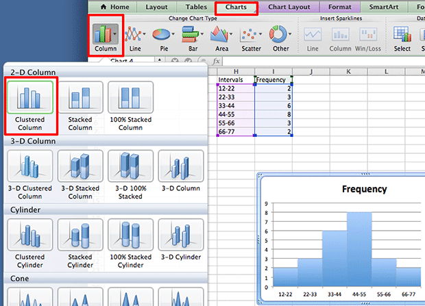
Create a Histogram Graph in Excel

Create Dynamic Chart Data Labels with Slicers - Excel Campus Feb 10, 2016 · Repeat this step for each series in the chart. If you are using Excel 2010 or earlier the chart will look like the following when you open the file. ... This table contains the three options for the different data labels. ... [on the use of Excel]. The problem with the graph is that there is too much detail being presented – we need to show ...

Share :